Euler Method
Goal of This Page
Understand the recurrence formula of the forward Euler method and the geometric meaning of tangent approximation, and learn the concepts of error order, stability, and implicit methods.
Prerequisites
- Chapter 9: Truncation Error
- Basics of ordinary differential equations (initial value problems)
- Basics of Taylor series
1. Problem Setting
Consider the initial value problem (IVP: Initial Value Problem):
\begin{equation} \dfrac{dy}{dx} = f(x, y), \qquad y(x_0) = y_0 \label{eq:ivp} \end{equation}Integrating both sides from $x_n$ to $x_{n+1}$ yields
$$y(x_{n+1}) = y(x_n) + \displaystyle\int_{x_n}^{x_{n+1}} f\bigl(x,\, y(x)\bigr)\, dx$$The integral representation on the right-hand side is exact, but the unknown function $y(x)$ appears inside the integrand, so in general this formula alone cannot be used to compute the value directly (many equations, such as linear or separable ones, do have analytical solutions, but those are obtained by other means). Approximating this integral by some means is therefore the fundamental idea behind numerical methods.
When the solution cannot be obtained analytically, it is necessary to construct an approximate solution numerically. Divide the interval $[x_0, x_0 + L]$ into equally spaced subintervals:
$$x_n = x_0 + nh, \quad n = 0, 1, 2, \dots, N, \qquad h = \dfrac{L}{N}$$and compute the approximation $y_n$ to $y(x_n)$ at each grid point $x_n$ successively.
![Equal spacing of the interval [x0, x0+L] with grid points](fig-grid-points.svg)
2. Forward Euler Method (Explicit Euler Method)
Starting from the initial value $y_0$, compute $y_1, y_2, \dots$ successively by the following recurrence:
$$y_{n+1} = y_n + h \cdot f(x_n, y_n)$$2.1 Derivation
The method can be derived from the Taylor expansion. For the exact solution $y(x)$,
$$y(x_{n+1}) = y(x_n) + h \, y'(x_n) + \dfrac{h^2}{2} y''(x_n) + O(h^3) = y(x_n) + h \, f(x_n, y(x_n)) + O(h^2)$$Dropping the $O(h^2)$ terms yields the forward Euler recurrence.
The same result can also be obtained from the integral perspective. In the integral form from Section 1, approximating the integrand $f(x, y(x))$ on the interval $[x_n, x_{n+1}]$ by its value at the left endpoint $f(x_n, y(x_n))$ (the left-rectangle rule), and then replacing the unknown $y(x_n)$ by the approximation $y_n$ to obtain $f(x_n, y_n)$, gives
$$\displaystyle\int_{x_n}^{x_{n+1}} f(x,\, y(x))\, dx \approx h \cdot f(x_n, y_n)$$which yields the forward Euler recurrence. In other words, the forward Euler method amounts to approximating $f$ by a step function on each subinterval and integrating.
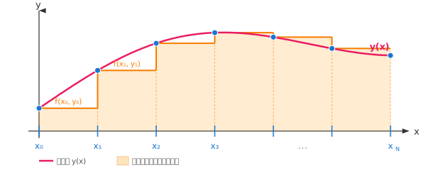
2.2 Geometric Interpretation
The integral perspective above can be rephrased geometrically as follows. From equation $\eqref{eq:ivp}$, $f(x, y) = dy/dx$, so $f(x_n, y_n)$ is the value of the slope field (vector field) at the point $(x_n, y_n)$, that is, the slope of the tangent line to the solution curve passing through that point. Note that the approximation $y_n$ generally differs from the exact value $y(x_n)$, so this solution curve is not the exact solution of the initial value problem itself but the solution curve through $(x_n, y_n)$ (the two coincide for $n = 0$). Thus, "approximating $f$ by its value at the left endpoint" amounts to replacing that solution curve by its tangent line and proceeding along it.
In other words, the forward Euler method advances along the tangent line at the point $(x_n, y_n)$ by the step size $h$, and takes the resulting point as the next approximation $y_{n+1}$. Advancing $h$ in the $x$-direction produces a change of $h \cdot f(x_n, y_n)$ in the $y$-direction.
An important observation regarding Figure 3: the slope of each blue line segment is not the slope of the exact solution (green curve), but the slope $f(x_n, y_n)$ computed from the approximate value $y_n$. In the first interval $[x_0, x_1]$, we have $y_0 = y(x_0)$, so the two slopes coincide. From the second interval onward, however, the approximate value $y_n$ deviates from the exact value $y(x_n)$, causing the blue segments to have a different slope from the exact solution. Even in the first interval, however, there is already an error from approximating a finite interval by a straight tangent segment (the local truncation error, Section 3.1). This "error of approximating an interval by the tangent" and, from the second interval onward, the "error of evaluating the slope at a displaced approximate point" combine and accumulate into the global error.
2.3 Worked Example
Solve $y' = y$, $y(0) = 1$ (exact solution $y = e^x$) with $h = 0.5$ up to $x = 2$.
| $n$ | $x_n$ | $y_n$ (Euler) | $y(x_n)$ (Exact) | Error |
|---|---|---|---|---|
| 0 | 0.0 | 1.0000 | 1.0000 | 0.0000 |
| 1 | 0.5 | 1.5000 | 1.6487 | 0.1487 |
| 2 | 1.0 | 2.2500 | 2.7183 | 0.4683 |
| 3 | 1.5 | 3.3750 | 4.4817 | 1.1067 |
| 4 | 2.0 | 5.0625 | 7.3891 | 2.3266 |
With $h = 0.5$ the error is large, but reducing $h$ improves accuracy. Comparing the error at $x = 2$ for different step sizes:
| $h$ | Steps | $y_N$ (Euler) | Error |
|---|---|---|---|
| 0.5 | 4 | 5.0625 | 2.3266 |
| 0.1 | 20 | 6.7275 | $6.6 \times 10^{-1}$ |
| 0.01 | 200 | 7.3160 | $7.3 \times 10^{-2}$ |
| 0.001 | 2,000 | 7.3817 | $7.4 \times 10^{-3}$ |
| 0.0001 | 20,000 | 7.3883 | $7.4 \times 10^{-4}$ |
Reducing $h$ by a factor of 10 reduces the error by roughly a factor of 10 (from the first row to the second, $h$ goes from $0.5$ to $0.1$, a factor of 5, so the error ratio is only about 3.5). This reflects the fact that the Euler method is first-order accurate ($O(h)$). Note, however, that this is an asymptotic property as $h \to 0$; it does not hold for coarse $h$ outside the stability region discussed later (Section 5.3).
Is smaller $h$ always better? From the viewpoint of truncation error, smaller $h$ yields better accuracy, but there are practical limits.
- Accumulation of roundoff errors: If $h$ is extremely small, the number of steps becomes enormous and floating-point roundoff errors accumulate. At some point, the decrease in truncation error and the increase in roundoff error balance out, and reducing $h$ further does not improve accuracy. A rough guide is the $h$ at which the truncation error $\sim Ch$ and the roundoff error $\sim \varepsilon\sqrt{L/h}$ ($\varepsilon$ is the machine epsilon) balance; for the example in this section this is around $h \sim 10^{-11}$ in double precision and $h \sim 10^{-5}$ in single precision. For the range of $h$ normally used in double precision, computation time becomes a problem well before this plateau.
- Computational cost: Halving $h$ doubles the computational cost. Balancing accuracy and computational cost is essential.
When high accuracy is required, rather than making $h$ arbitrarily small, it is more efficient to use a higher-order method such as the Runge-Kutta method.
3. Error Analysis
3.1 Local Truncation Error
The local truncation error is the error introduced in a single step, defined by assuming departure from the exact solution:
$$\tau_n = y(x_{n+1}) - \bigl[y(x_n) + h f(x_n, y(x_n))\bigr] = \dfrac{h^2}{2} y''(\xi_n) = O(h^2)$$Since the $O(h^2)$ term in the Taylor expansion is truncated, the local truncation error is $O(h^2)$.
3.2 Global Error
The global error is defined as $e_n = y(x_n) - y_n$. The following assumes that $f$ is Lipschitz continuous in $y$ (with constant $L_f$) and that the solution $y$ is twice continuously differentiable on the finite interval $[x_0, x_0 + L]$ (the expression $\tau_n = \tfrac{h^2}{2} y''(\xi_n)$ in Section 3.1 also requires $y \in C^2$). Then, due to the accumulation over $N = L/h$ steps,
$$|e_N| \le C \cdot h$$That is, the global error is $O(h)$. This is why the Euler method is said to be a first-order method. Intuitively, the local error of $O(h^2)$ accumulates over $N = O(1/h)$ steps, giving $O(h^2) \times O(1/h) = O(h)$. However, the local errors are not simply added up: they accumulate while being amplified by the subsequent steps. The constant $C$ has the form $\dfrac{\max|y''|}{2L_f}\bigl(e^{L_f L} - 1\bigr)$, which grows exponentially with the interval length $L$ and the Lipschitz constant $L_f$, so $C$ itself can become very large on long intervals. Indeed, for the example of Section 2.3 ($y' = y$, $[0, 2]$, $h = 0.001$), the global error is about 2.3 times the sum of the local errors.
In general, for a one-step method whose error propagation is stable, a local truncation error of $O(h^{p+1})$ per step leads to a global error of $O(h^p)$ ($p$-th order accuracy). The order of the local error alone is not sufficient; stable error propagation (e.g., the Lipschitz condition above) is also required.
4. Backward Euler Method (Implicit Euler Method)
$y_{n+1} = y_n + h \cdot f(x_{n+1}, y_{n+1})$
From the integral perspective, whereas the forward Euler method corresponds to the left-rectangle rule (approximating $f$ by its value at the left endpoint of the interval), the backward Euler method corresponds to the right-rectangle rule (approximating $f$ by its value at the right endpoint $f(x_{n+1}, y_{n+1})$):
$$\displaystyle\int_{x_n}^{x_{n+1}} f(x,\, y(x))\, dx \approx h \cdot f(x_{n+1}, y_{n+1})$$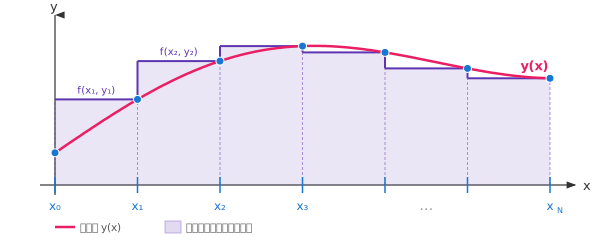
Since the unknown $y_{n+1}$ appears on the right-hand side, for a general nonlinear $f$ a nonlinear equation in $y_{n+1}$ must be solved at each step (typically using an iterative method such as Newton's method). If $f$ is linear in $y$, only a linear equation is needed, and as with the test equation it can sometimes be solved explicitly. The computational cost is higher than the forward Euler method, but the stability is superior.
4.1 Why Is the Stability Superior?
The intuitive reason can be seen with the decaying solution $y' = \lambda y$ ($\lambda < 0$). The exact solution decays as $y = e^{\lambda x} \to 0$.
The forward Euler method determines the next value based on "old information" $y_n$:
$$y_{n+1} = (1 + h\lambda)\, y_n$$When $\lambda < 0$, if $h$ is too large, $|1 + h\lambda| > 1$ and the solution, which should be decaying, oscillates and diverges. For example, with $\lambda = -10$ and $h = 0.3$, $1 + h\lambda = 1 - 3 = -2$, and $|y_n|$ doubles at every step.
The backward Euler method determines the value using "information at the destination" $y_{n+1}$:
$$y_{n+1} = y_n + h\lambda\, y_{n+1} \implies y_{n+1} = \dfrac{y_n}{1 - h\lambda}$$When $\lambda < 0$ and $h > 0$, $1 - h\lambda = 1 + h|\lambda| > 1$, so $|y_{n+1}| < |y_n|$ always holds. No matter how large $h$ is, the solution decays and never diverges. This is the essence of the stability of the backward Euler method. Note, however, that this is a stability property; it does not mean that accuracy is preserved when $h$ is made large (Section 5.3).
In other words, the forward Euler method overshoots in rapidly changing situations by using the "old slope," whereas the backward Euler method automatically applies a brake via the "slope at the destination." The stiff equations for which this property is particularly important are discussed in Section 5.3.
5. Stability Analysis
To investigate stability, we use the test equation $y' = \lambda y$ ($\mathrm{Re}(\lambda) < 0$). The exact solution is $y = e^{\lambda x} \to 0$ ($x \to \infty$), and it is desirable for the numerical solution to reproduce this decay.
5.1 Forward Euler Method
Since $y_{n+1} = (1 + h\lambda) y_n$, the amplification factor is $R(z) = 1 + z$ ($z = h\lambda$). For $|y_n| \to 0$, the condition
$$|1 + z| < 1$$must hold. This corresponds to the interior of a circle centered at $(-1, 0)$ with radius $1$ in the complex plane, known as the stability region. When $\lambda$ is a large negative real number, the step size restriction $h < 2/|\lambda|$ applies.
5.2 Backward Euler Method
Since $y_{n+1} = \dfrac{1}{1 - z} y_n$, the stability condition is $|1/(1-z)| < 1$, i.e., $|1 - z| > 1$. When $\mathrm{Re}(\lambda) < 0$, this condition is satisfied for all $h > 0$. That is, the stability region of the backward Euler method contains the entire left half of the complex plane $\{z : \mathrm{Re}(z) < 0\}$; such a method is called A-stable. A-stability is the property that, for the test equation, the method is stable for any $h > 0$ whenever $\mathrm{Re}(\lambda) < 0$; it does not guarantee stability or accuracy for arbitrary nonlinear problems.
5.3 Stiff Equations and Advantages of the Backward Euler Method
Equations that contain components with vastly different time constants, so that accuracy alone would permit a large step size but the rapidly decaying component forces a severe stability restriction on the step size of explicit methods, are called stiff equations. Stiffness is not the size of a coefficient as such; it shows up as this situation in which stability, not accuracy, dictates the step size. For example, in $y_1' = -y_1,\ y_2' = -1000 y_2$, following the slow component $y_1$ requires an interval of length of order 1 in $x$, but the forward Euler method is forced to take $h < 2/|\lambda| = 0.002$ because of the fast component $y_2$ ($\lambda = -1000$). At exactly $h = 0.002$ the method does not diverge, but an oscillation of amplitude $\pm 1$ persists forever and the decay is not reproduced; for larger $h$ it diverges. Even the scalar equation $y' = -1000y$ presents the same difficulty when its decay is far faster than the time scale of interest ($x \sim 1$).
The backward Euler method, on the other hand, remains stable for any $h$. Although the cost per step is higher, the ability to take much larger step sizes greatly reduces the total number of steps, resulting in better overall efficiency. This is the advantage of the backward Euler method (and implicit methods in general) for stiff equations. However, the accuracy of the backward Euler method is first order ($O(h)$), the same as the forward Euler method, so being able to take a large $h$ means "the solution does not blow up," not "the required accuracy is achieved." For example, advancing $y' = -10y$, $y(0) = 1$ to $x = 1$ in a single step with $h = 1$ gives $1/11 \approx 0.091$, which does not diverge but is about 2000 times the exact value $e^{-10} \approx 4.5 \times 10^{-5}$. The step size is ultimately determined by the accuracy requirement.
Moreover, the global error $O(h)$ of Section 3.2 is an asymptotic statement as $h \to 0$ and does not hold while $h$ lies outside the stability region. Solving $y' = -1000y$ up to $x = 0.01$, even after $h$ drops below the stability limit $0.002$, "halving $h$ halves the error" does not hold for a while (halving $h = 1.25 \times 10^{-3}$ actually increases the error); the error ratio only exceeds 1.9 and approaches 2 once $h$ is below roughly $3 \times 10^{-5}$.
6. Improved Euler Method (Heun's Method)
Compute $y_{n+1}$ in the following two stages:
$$\tilde{y}_{n+1} = y_n + h \, f(x_n, y_n) \qquad \text{(predictor: forward Euler)}$$ $$y_{n+1} = y_n + \dfrac{h}{2} \bigl[f(x_n, y_n) + f(x_{n+1}, \tilde{y}_{n+1})\bigr] \qquad \text{(corrector: trapezoidal rule)}$$From the integral perspective, this uses the idea of the trapezoidal rule, which approximates $f$ by the average of its values at the left and right endpoints. At the right endpoint, however, the predictor $\tilde{y}_{n+1}$ is used instead of the unknown $y_{n+1}$:
$$\displaystyle\int_{x_n}^{x_{n+1}} f(x,\, y(x))\, dx \approx \dfrac{h}{2}\bigl[f(x_n, y_n) + f(x_{n+1}, \tilde{y}_{n+1})\bigr]$$Using $y_{n+1}$ itself at the right endpoint gives a different method, the implicit trapezoidal method (A-stable, second order). Heun's method replaces $y_{n+1}$ by the predictor $\tilde{y}_{n+1}$ to make the method explicit, at the cost of losing A-stability (see the table in Section 7).
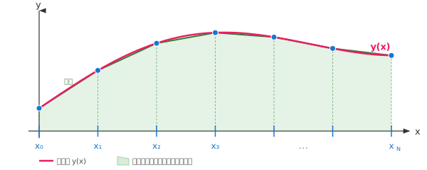
Since the trapezoidal approximation follows the curve more closely than the rectangular approximation, accuracy is improved:
- Local truncation error: $O(h^3)$
- Global error: $O(h^2)$ (second-order accuracy)
The improved Euler method is a type of two-stage, second-order Runge-Kutta method (RK2). Although explicit, it achieves twice the order of accuracy of the forward Euler method. The computational cost per step is two evaluations of $f$ (twice that of the forward Euler method), but since the step size required to achieve the same accuracy can be made considerably larger, the improved Euler method is often more efficient overall.
7. Comparison of Methods
Comparing the characteristics of the three methods described here (forward Euler, backward Euler, improved Euler = Heun's method) and the classical four-stage, fourth-order method (RK4) among the Runge-Kutta methods discussed on a separate page, we obtain the following table. Runge-Kutta methods form a family; the order, number of stages, and stability differ from one scheme to another. The values in the table are those of RK4.
| Method | Local Error | Global Error | $f$ evals/step | A-stable |
|---|---|---|---|---|
| Forward Euler | $O(h^2)$ | $O(h)$ | 1 | No |
| Backward Euler | $O(h^2)$ | $O(h)$ | 1 + solve | Yes |
| Improved Euler | $O(h^3)$ | $O(h^2)$ | 2 | No |
| Classical 4th-order Runge-Kutta method (RK4) | $O(h^5)$ | $O(h^4)$ | 4 | No |
Comparing the relationship between step size $h$ and global error on a logarithmic scale for the four methods listed in the table above, the difference in order of accuracy of each method becomes clearly visible.

Since this figure uses $y' = y$ ($\lambda = 1$, a growing solution), the accuracy of the forward and backward Euler methods appears nearly identical. The main advantage of the backward Euler method lies not in its order of accuracy but in its stability: for stiff equations it allows much larger step sizes than explicit methods (see Section 5.3).
8. Frequently Asked Questions
Q1. Why is the error of the Euler method $O(h)$?
The local truncation error introduced in a single step of the Euler method is $O(h^2)$ (Section 3.1). Advancing across the interval $[x_0, x_0 + L]$ with step size $h$ requires $N = L/h = O(1/h)$ steps, and intuitively the $O(h^2)$ local error appears $O(1/h)$ times, so the resulting global error is $O(h^2) \times O(1/h) = O(h)$. Rigorously, the global error $O(h)$ is established by estimating the propagation (amplification) of the errors under a Lipschitz condition on $f$ (Section 3.2). The Euler method is therefore first-order accurate: for sufficiently small $h$, halving the step size $h$ roughly halves the error (see the numerical experiment in Section 2.3).
Q2. What is the difference between the local truncation error and the global error of the Euler method?
The local truncation error (LTE) is the error introduced in a single step starting from the exact solution; for the Euler method it is $\tau_n = \tfrac{h^2}{2} y''(\xi_n) = O(h^2)$. The global error (GTE) is the final error after $N$ steps from the initial value, $e_n = y(x_n) - y_n = O(h)$. The global error is the accumulation of the local truncation error over all steps; for a stable one-step method on a finite interval, a local truncation error of $O(h^{p+1})$ typically corresponds to a global error of $O(h^p)$ (the accumulation lowers the order by one). See Truncation Error for details.
Q3. How can I reduce the error of the Euler method?
Since the global error is $O(h)$, reducing the step size $h$ reduces the error proportionally. However, making $h$ extremely small leads to an enormous number of steps and accumulating roundoff error, so accuracy eventually plateaus (see the note in Section 2.3). When high accuracy is required, rather than shrinking $h$ indefinitely it is more efficient to use a higher-order method such as the improved Euler method (global error $O(h^2)$) or the Runge-Kutta method ($O(h^4)$).
Q4. What is the Euler method?
The Euler method is the most fundamental numerical method for the ordinary differential equation $y' = f(x, y)$; it computes an approximate solution by the recurrence $y_{n+1} = y_n + h \, f(x_n, y_n)$ (Section 2). Geometrically, at each approximate point $(x_n, y_n)$ it draws the tangent line (with slope $f(x_n, y_n)$) to the solution curve through that point and advances along it by the step size $h$ to obtain the next approximation (Section 2.2). From the integral perspective, it corresponds to approximating the integral of $f$ by the left-rectangle rule (Section 2.1).
Q5. What is the difference between the forward and backward Euler methods?
The forward Euler method (explicit) uses $y_{n+1} = y_n + h \, f(x_n, y_n)$ and computes the next value directly from known values (corresponding to the left-rectangle rule). The backward Euler method (implicit) uses $y_{n+1} = y_n + h \, f(x_{n+1}, y_{n+1})$, where the unknown $y_{n+1}$ also appears on the right-hand side, so an equation in $y_{n+1}$ (a nonlinear equation for general nonlinear $f$) must be solved at each step (corresponding to the right-rectangle rule). The backward Euler method is A-stable and can be applied to stiff equations (Sections 4 and 5).
Q6. How accurate is the Euler method?
The Euler method has a local truncation error of $O(h^2)$ (per step) and a global error of $O(h)$ (first-order accuracy) (Section 3). That is, for sufficiently small $h$, halving the step size roughly halves the error. Because of its low accuracy, higher-order methods such as the classical 4th-order Runge-Kutta method (RK4, global error $O(h^4)$) are used in practice, but the Euler method remains important as a theoretical foundation (Section 7).
References
- J. C. Butcher, Numerical Methods for Ordinary Differential Equations, 3rd ed., Wiley, 2016.
- E. Hairer, S. P. Nørsett, G. Wanner, Solving Ordinary Differential Equations I: Nonstiff Problems, 2nd ed., Springer, 1993.
- U. M. Ascher, L. R. Petzold, Computer Methods for Ordinary Differential Equations and Differential-Algebraic Equations, SIAM, 1998.
- Euler method — Wikipedia
Summary
Key Takeaways
- Forward Euler method: $y_{n+1} = y_n + hf(x_n, y_n)$ (tangent approximation)
- Local truncation error $O(h^2)$, global error $O(h)$ (first-order accuracy)
- Backward Euler method (implicit): generally requires solving an equation at each step; its stability region contains the left half-plane (A-stable)
- Stability is analyzed using the test equation $y' = \lambda y$ and the amplification factor $R(z)$ ($z = h\lambda$); the region of absolute stability is taken as $|R(z)| \le 1$
- Improved Euler method (Heun's method): second-order accuracy, more accurate than the forward Euler method