What is GMM (Gaussian Mixture Model)? Complete Derivation of the EM Algorithm
Gaussian Mixture Model & EM Algorithm
What is GMM?
Definition: GMM (Gaussian Mixture Model)
A Gaussian Mixture Model (GMM) is a probabilistic model that represents the probability distribution of data as a weighted sum of multiple normal (Gaussian) distributions.
Here, $K$ is the number of component distributions, $\pi_k$ is the mixing coefficient ($\pi_k\geq 0$ and $\sum_k \pi_k = 1$), $\boldsymbol{\mu}_k$ is the mean vector, and $\boldsymbol{\Sigma}_k$ is a symmetric positive definite covariance matrix. Throughout this article the normal density is written $N(\boldsymbol{x} \mid \boldsymbol{\mu},\boldsymbol{\Sigma})$.
Intuitive Understanding
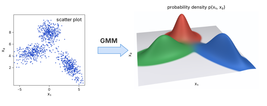
Consider a data distribution with multiple peaks that cannot be adequately represented by a single normal distribution. In a GMM, a latent variable first selects one of the components, and the distribution conditional on that component is normal. The resulting density is a weighted sum, with mixing coefficients $\pi_k$, of the normal distributions corresponding to the individual peaks, which flexibly approximates complex distributions. The parameters are estimated using the EM algorithm (Expectation-Maximization).
Fig. 1: Data generated from three normal distributions (left, a scatter plot), represented by a Gaussian mixture model (GMM). Each cluster becomes a single peak, and together they form the 3D probability-density surface $p(\boldsymbol{x})$ (right). A GMM flexibly approximates a multi-peaked distribution as a weighted sum of normal distributions that differ in orientation and spread.
Applications
Clustering: Unlike K-means, each data point can belong to multiple clusters with different probabilities (soft clustering)
Anomaly detection: Learn the density of normal data with a GMM and flag points in low-probability regions as anomalies
Speech recognition: Modeling the acoustic features of speakers
Density estimation: As a parametric alternative to kernel density estimation
GMM vs K-means vs Kernel Density Estimation
Feature
GMM
K-means
Kernel Density Estimation
Cluster assignment
Soft (probabilistic)
Hard (single cluster)
—
Cluster shape
Elliptical (arbitrary covariance)
Isotropic (spherical) assumed
—
Probabilistic model
Yes (generative model)
No
Yes (nonparametric)
Number of parameters
$O(KD^2)$
$O(KD)$
$O(ND)$ (depends on data size)
Estimation method
EM algorithm
Lloyd's algorithm
Bandwidth selection
Introduction (Scope of This Article)
Building on the overview of GMM presented above, this article provides a complete derivation without skipping any intermediate steps of the parameter estimation via the EM algorithm.
Specifically, for each of the mean vector, the covariance matrix, and the mixing coefficients, we rigorously derive the stationarity conditions from the partial derivatives of the log-likelihood function using matrix calculus and obtain the parameter update formulas.
For the covariance matrix, we adopt the approach of working through the precision matrix (the inverse), combining the derivative of the determinant with the derivative of the quadratic form.
The mixing coefficients are estimated via constrained optimization using the method of Lagrange multipliers, and finally, we present a convergence proof of the EM algorithm based on the ELBO (Evidence Lower Bound) and the KL divergence.
Throughout this article, boldface denotes vectors or matrices, and for a matrix $\boldsymbol{A}$, we write $\boldsymbol{A}^{-T}=\left(\boldsymbol{A}^{-1}\right)^T$ for the transpose of its inverse.
Normal Distribution
The $D$-dimensional normal distribution, parameterized by a mean vector $\boldsymbol{\mu}\in\mathbb{R}^D$ and a symmetric positive definite covariance matrix $\boldsymbol{\Sigma}\in\mathbb{R}^{D\times D}$, is given by the formula below. Without positive definiteness one cannot conclude $|\boldsymbol{\Sigma}|>0$, so $|\boldsymbol{\Sigma}|^{-\frac{1}{2}}$ need not be real, and the exponent is unbounded above, so the density fails to be integrable.
We define the Gaussian mixture distribution as a linear combination of normal distributions $N(\boldsymbol{x}|\boldsymbol{\mu},\boldsymbol{\Sigma})$ as follows.
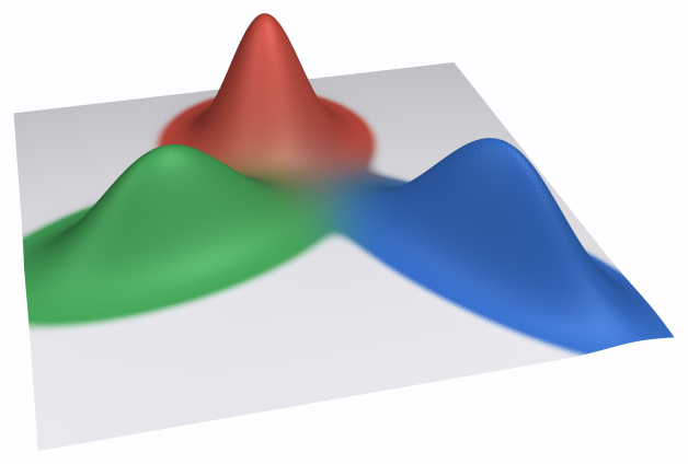
Fig. 2: Density surface of a $K=3$ Gaussian mixture $p(\boldsymbol{x})=\displaystyle\sum_{k=1}^{3}\pi_k N(\boldsymbol{x}|\boldsymbol{\mu}_k,\boldsymbol{\Sigma}_k)$.
Each component $\pi_k N(\boldsymbol{x}|\boldsymbol{\mu}_k,\boldsymbol{\Sigma}_k)$ forms one bump; the mixing coefficient $\pi_k$ and covariance $\boldsymbol{\Sigma}_k$ set its height and spread. Color shows the responsibility (posterior probability) $\gamma_{n,k}=\dfrac{\pi_k N(\boldsymbol{x}_n|\boldsymbol{\mu}_k,\boldsymbol{\Sigma}_k)}{\displaystyle\sum_j \pi_j N(\boldsymbol{x}_n|\boldsymbol{\mu}_j,\boldsymbol{\Sigma}_j)}$ of each component, blending the component colors (red/blue/green). Where the components overlap the assignment is probabilistic, and the color boundaries are the decision boundaries obtained by hard-assigning each point to the component with the largest responsibility.
The mixing coefficients $\pi_k$ correspond to probabilities and satisfy
Assuming the observed samples $\boldsymbol{x}_n\in\mathbb{R}^D,\ n=1,2,3,\cdots N$ are generated from the Gaussian mixture model in Eq.(\ref{GMM}), we seek parameters $\boldsymbol{\pi},\boldsymbol{\mu},\boldsymbol{\Sigma}$ that make the log-likelihood function large
Note that this log-likelihood function is not bounded above: if the mean of one component is placed at a single data point and that component's covariance matrix is allowed to degenerate, the log-likelihood grows without bound (a degenerate solution), so no global maximum exists.
What we derive below is therefore a stationary point satisfying the first-order necessary condition (zero gradient); second-order conditions are not treated. In practice one avoids the degenerate solutions by regularization or by a careful choice of initial values, and looks for a meaningful stationary point.
Here, $\boldsymbol{X}$ denotes the data matrix representing the sample set $\{\boldsymbol{x}_1, \boldsymbol{x}_2, \cdots \boldsymbol{x}_N\}$.
Let $z_n \in \{1, 2, \cdots, K\}$ be a latent variable indicating which normal distribution generated the sample $\boldsymbol{x}_n$, and let $P(z_n = m) = \pi_m$.
The posterior probability that the sample $\boldsymbol{x}_n$ was generated by the $m$-th normal distribution can be computed using Bayes' theorem as
Since the sample $\boldsymbol{x}_n$ was generated by one of the $K$ normal distributions, summing $\gamma_{n,m}$ over $m=1,2,3,\cdots K$ naturally yields a total probability of 1.
Deriving $\boldsymbol{\mu}_m$ from the Stationarity Condition
In this section, we differentiate the log-likelihood function with respect to the mean vector and apply the vector derivative of a quadratic form to solve the stationarity condition.
The result shows that the mean vector of each cluster is the responsibility-weighted average of the samples.
The following derivation adopts the denominator layout convention: the derivative of a scalar function with respect to a vector is a column vector.
Differentiating the log-likelihood function with respect to $\boldsymbol{\mu}_m$, we obtain
Deriving $\boldsymbol{\Sigma}_m$ from the Stationarity Condition
In this section, we solve the stationarity condition for the covariance matrix.
Since direct differentiation is difficult, we reparameterize the log-likelihood in terms of the precision matrix (the inverse), and combine the derivative of the log-determinant with the derivative of the outer-product quadratic form to obtain the solution.
The result is the responsibility-weighted mean of the outer products of the deviations.
Since $\boldsymbol{\Sigma}_m$ is symmetric positive definite, so is the precision matrix $\boldsymbol{\Gamma}_m=\boldsymbol{\Sigma}_m^{-1}$, and $|\boldsymbol{\Gamma}_m|^{\frac{1}{2}}$ is a well-defined real number.
In what follows we differentiate treating all $D^2$ entries of $\boldsymbol{\Gamma}_m$ as independent. Imposing the symmetry constraint doubles the rate of change of the off-diagonal entries, but it does not move the points where the gradient vanishes, so the stationarity condition gives the same result.
Let the inverse of the covariance matrix $\boldsymbol{\Sigma}_m$ be
can be obtained by solving the equation below. This is because $\boldsymbol{\Sigma}\mapsto\boldsymbol{\Sigma}^{-1}$ is a bijection on the set of symmetric positive definite matrices whose derivative is nonsingular, so by the chain rule the points where one gradient vanishes coincide with the points where the other does.
Since in general $\{f(\boldsymbol{x})g(\boldsymbol{x})\}'=f'(\boldsymbol{x})g(\boldsymbol{x})+f(\boldsymbol{x})g'(\boldsymbol{x})$, the expression after $\displaystyle\frac{\partial}{\partial\boldsymbol{\Gamma}_m}$ can be written as
In this section, we solve the stationarity condition for the mixing coefficients.
Since the mixing coefficients are subject to the equality constraint that they sum to 1, we formulate the problem as constrained optimization using the method of Lagrange multipliers and eliminate the multiplier to obtain a closed-form solution.
The mixing coefficients $\pi_m$ must satisfy the strong constraint $\displaystyle\sum_{m=1}^K \pi_m=1$. We therefore use the method of Lagrange multipliers and look for stationary points of the log-likelihood function augmented by the term $\lambda\left(\displaystyle\sum_{k=1}^K \pi_k -1\right)$.
In what follows we assume an interior solution with $\pi_m>0$. The stationarity condition involves $1/\pi_m$, so the derivation does not apply at the boundary $\pi_m=0$, and for an empty component with $N_m=0$ the update itself is undefined (an implementation removes or reinitializes such a component).
The inequality constraint $0\leq\pi_k\leq 1$ need not be imposed separately: the resulting $\pi_m=N_m/N$ satisfies it automatically because $\gamma_{n,m}\geq 0$ and $\displaystyle\sum_{m=1}^K N_m=N$.
Since $\displaystyle\sum_{n=1}^N \gamma_{n,m}$ can be interpreted as the estimated number of samples generated by the $m$-th normal distribution, we write it as $N_m$ for a more compact notation.
However, since the formula for $\gamma_{n,m}$ contains $\boldsymbol{\mu}_m, \boldsymbol{\Sigma}_m, \pi_m$, and the formulas for $\boldsymbol{\mu}_m, \boldsymbol{\Sigma}_m, \pi_m$ contain $\gamma_{n,m}$, this system of equations is nonlinear and cannot be solved in closed form. We therefore adopt the EM algorithm, which starts from initial values and alternates between the E-step and M-step, keeping the log-likelihood non-decreasing while approaching a stationary point that depends on those initial values.
Procedure of the EM Algorithm
Set initial values $\boldsymbol{\mu}_m^{(0)}, \boldsymbol{\Sigma}_m^{(0)}, \pi_m^{(0)}$ and let $i=0$.
Using $\boldsymbol{\mu}_m^{(i)}, \boldsymbol{\Sigma}_m^{(i)}, \pi_m^{(i)}$, compute $\gamma_{n,m}^{(i)}$ and $N_m^{(i)}$ (E-step):
Using $\gamma_{n,m}^{(i)}$ and $N_m^{(i)}$, update the parameters $\boldsymbol{\mu}_m^{(i+1)}, \boldsymbol{\Sigma}_m^{(i+1)}, \pi_m^{(i+1)}$ (M-step). The covariance uses the updated $\boldsymbol{\mu}_m^{(i+1)}$ computed first:
If sufficiently converged, terminate. Otherwise, set $i\leftarrow i+1$ and return to Step 2.
Fig. 3: The EM algorithm running on the scatter data of Fig. 1. At the initial guess (iteration 0) the three isotropic Gaussians sit in the wrong places, but with each E-step and M-step they translate, rotate and rescale to lock onto the three clusters. Each point is coloured by its responsibilities $\gamma_{n,m}$ at that iteration (a blend of the three component colours), so the assignment sharpens as it converges. The log-likelihood is non-decreasing at every iteration. Use Prev / Auto / Next (or the slider) to step through the iterations.
Caution
The EM algorithm is not guaranteed to converge to the global optimum from an arbitrary initial point.
In addition, for a component with a small $N_m^{(i)}$ the updated $\boldsymbol{\Sigma}_m^{(i+1)}$ can approach a singular matrix, breaking the computation of $\boldsymbol{\Sigma}_m^{-1}$ and $|\boldsymbol{\Sigma}_m|$. Implementations keep it positive definite, for instance by adding a small $\varepsilon\boldsymbol{I}$ to $\boldsymbol{\Sigma}_m$ (see Convergence of the EM Algorithm).
On the $\boldsymbol{\mu}_m$ Used in the Covariance Update
In the computation of $\boldsymbol{\Sigma}_m^{(i+1)}$ in Eq.(\ref{update}), we use $\boldsymbol{\mu}_m^{(i+1)}$, the value updated earlier in the same M-step.
This is the solution that maximizes the $Q$ function jointly over $\boldsymbol{\mu}_m$ and $\boldsymbol{\Sigma}_m$ with the responsibilities $\gamma_{n,m}^{(i)}$ held fixed, and it is the standard EM update. Major libraries such as scikit-learn adopt this form.
A variant that uses the old value $\boldsymbol{\mu}_m^{(i)}$ instead is also seen.
That variant is not the joint maximizer of $Q$; it can be viewed as an instance of the ECM (Expectation Conditional Maximization) algorithm [Meng & Rubin, 1993], in which the M-step performs conditional maximization in the order $\boldsymbol{\Sigma}_m \to \boldsymbol{\mu}_m$.
The standard convergence proof of EM relies on the M-step maximizing all parameters simultaneously, so it does not directly apply to such a sequential update.
However, Meng & Rubin (1993) proved that if each conditional maximization step increases $Q$, then the log-likelihood is non-decreasing overall, so monotonicity is preserved for the variant as well.
The two updates do not necessarily converge to the same point; depending on the initial values they can settle on different local optima.
Convergence of the EM Algorithm
In this section, we prove that the log-likelihood monotonically increases (more precisely, is non-decreasing) at each iteration of the EM algorithm.
We decompose the log-likelihood into the ELBO (Evidence Lower Bound) and the KL divergence, and show that the E-step sets the KL divergence to zero while the M-step maximizes the ELBO, thereby ensuring the log-likelihood improves at each iteration.
We show that the log-likelihood monotonically increases (is non-decreasing) at each iteration of the EM algorithm.
Lower Bound of the Log-Likelihood
Let $\boldsymbol{\theta}=\{\boldsymbol{\pi},\boldsymbol{\mu},\boldsymbol{\Sigma}\}$ denote the set of parameters and $\boldsymbol{Z}=\{z_1, z_2, \cdots, z_N\}$ the set of latent variables.
For any probability distribution $q(\boldsymbol{Z})$ over the latent variables $\boldsymbol{Z}$, the log-likelihood can be decomposed as follows.
$\mathcal{L}(q,\boldsymbol{\theta})$ is called the Evidence Lower Bound (ELBO), also known as the negative variational free energy.
The fundamental idea of the EM algorithm is to maximize this lower bound instead of the log-likelihood $\log p(\boldsymbol{X}|\boldsymbol{\theta})$, which is difficult to maximize directly.
$\mathrm{KL}(q \| p)$ is the Kullback-Leibler divergence (KL divergence) between $q(\boldsymbol{Z})$ and the posterior distribution $p(\boldsymbol{Z}|\boldsymbol{X},\boldsymbol{\theta})$, which always satisfies $\mathrm{KL}(q \| p) \geq 0$ (with equality when $q(\boldsymbol{Z}) = p(\boldsymbol{Z}|\boldsymbol{X},\boldsymbol{\theta})$).
Therefore, $\mathcal{L}(q,\boldsymbol{\theta})$ is a lower bound on the log-likelihood.
This inequality means that $\mathcal{L}(q,\boldsymbol{\theta})$ is always less than or equal to the log-likelihood.
Direct maximization of $\log p(\boldsymbol{X}|\boldsymbol{\theta})$ is difficult (because the $\sum$ is inside the $\log$), but by maximizing the lower bound $\mathcal{L}(q,\boldsymbol{\theta})$, we can indirectly increase the log-likelihood.
This is the fundamental idea behind the EM algorithm.
Interpretation of the E-step
In the E-step, we fix the current parameters $\boldsymbol{\theta}^{(i)}$ and find the $q(\boldsymbol{Z})$ that maximizes the lower bound $\mathcal{L}(q,\boldsymbol{\theta}^{(i)})$.
In $\log p(\boldsymbol{X}|\boldsymbol{\theta}^{(i)}) = \mathcal{L}(q,\boldsymbol{\theta}^{(i)}) + \mathrm{KL}(q \| p)$, the left-hand side does not depend on $q$, so maximizing $\mathcal{L}$ is equivalent to minimizing $\mathrm{KL}(q \| p)$.
Since $\mathrm{KL}(q \| p) \geq 0$ with equality when $q(\boldsymbol{Z}) = p(\boldsymbol{Z}|\boldsymbol{X},\boldsymbol{\theta}^{(i)})$, the optimal solution of the E-step is
In the M-step, we fix $q^{(i)}(\boldsymbol{Z})$ obtained in the E-step and find the parameters $\boldsymbol{\theta}^{(i+1)}$ that maximize the lower bound $\mathcal{L}(q^{(i)},\boldsymbol{\theta})$.
By maximization, we have $\mathcal{L}(q^{(i)},\boldsymbol{\theta}^{(i+1)}) \geq \mathcal{L}(q^{(i)},\boldsymbol{\theta}^{(i)})$.
Eq.(\ref{update}) in the section EM Algorithm is precisely the solution of this maximization over $\boldsymbol{\mu}_m,\boldsymbol{\Sigma}_m,\pi_m$ with the responsibilities fixed at $\gamma_{n,m}^{(i)}$. That is why $\boldsymbol{\Sigma}_m^{(i+1)}$ uses the updated $\boldsymbol{\mu}_m^{(i+1)}$: the variant that uses the old value $\boldsymbol{\mu}_m^{(i)}$ is not this $\arg\max$, so the proof below does not apply to it as it stands (see the note in the previous section).
Monotonic Increase of the Log-Likelihood
From the above, tracking the change in log-likelihood at each iteration gives
\begin{eqnarray}
\log p(\boldsymbol{X}|\boldsymbol{\theta}^{(i+1)})
&=& \mathcal{L}(q^{(i)},\boldsymbol{\theta}^{(i+1)}) + \mathrm{KL}(q^{(i)} \| p(\cdot|\boldsymbol{X},\boldsymbol{\theta}^{(i+1)})) \\
&\geq& \mathcal{L}(q^{(i)},\boldsymbol{\theta}^{(i+1)}) \\
&& \text{Since the lower bound was maximized in the M-step,} \nonumber \\
&\geq& \mathcal{L}(q^{(i)},\boldsymbol{\theta}^{(i)}) \\
&& \text{Since } \mathrm{KL}=0 \text{ was set in the E-step,} \nonumber \\
&=& \log p(\boldsymbol{X}|\boldsymbol{\theta}^{(i)})
\end{eqnarray}
Therefore, the log-likelihood monotonically increases (is non-decreasing) at each iteration of the EM algorithm.
If singular solutions are excluded by regularizing the covariance matrix (e.g., adding $\varepsilon\boldsymbol{I}$ to $\boldsymbol{\Sigma}_m$), the log-likelihood is bounded above, so the sequence of log-likelihood values, being non-decreasing and bounded above, converges.
Here $\varepsilon$ must be small compared with the scale of the data: if it is large, the M-step no longer maximizes $Q$ and the monotonicity argument used above breaks down (monotonicity is retained if the M-step is instead formulated as maximizing $Q$ subject to $\boldsymbol{\Sigma}_m \succeq \varepsilon\boldsymbol{I}$).
Convergence of the value sequence does not imply convergence of the parameter sequence itself, which requires additional conditions.
Moreover, there is no guarantee that the convergence point is the global optimum; convergence to a local optimum or a saddle point is possible.
Frequently Asked Questions
Q1. What is a Gaussian Mixture Model (GMM)?
A Gaussian Mixture Model (GMM) is a probabilistic model that represents the probability distribution of data as a weighted sum of multiple normal (Gaussian) distributions. Each component distribution is parameterized by a mean vector, a covariance matrix, and a mixing coefficient, which are estimated using the EM algorithm.
Q2. What are the applications of GMM?
GMMs are widely used in clustering (automatic data classification), anomaly detection, speech recognition (speaker modeling), image segmentation, and density estimation. Unlike K-means, GMM supports soft clustering, where each data point can belong to multiple clusters with different probabilities.
Q3. What is the difference between GMM and K-means?
K-means is a hard clustering method that assigns each data point to exactly one cluster; because it relies on Euclidean distance, it works best when the clusters are isotropic and of similar size. GMM is a soft clustering method that computes the probability of each data point belonging to each cluster and can represent elliptical clusters of varying sizes and orientations.
Q4. What is the EM algorithm?
The EM (Expectation-Maximization) algorithm is an iterative method for maximum likelihood estimation in probabilistic models with latent variables. It alternates between the E-step (computing the responsibilities of each data point) and the M-step (updating the parameters). The log-likelihood is non-decreasing at every iteration, but the point it converges to depends on the initial values and is not necessarily the global optimum.
C.M. Bishop, "Pattern Recognition and Machine Learning", Springer, 2006
X.L. Meng and D.B. Rubin, "Maximum Likelihood Estimation via the ECM Algorithm: A General Framework", Biometrika, 80(2), pp.267-278, 1993
📚 Studying statistics & machine learning from books? Reading Forest is a free reading-log app that records what you read and reminds you to review it at the right time — spaced repetition based on the Ebbinghaus forgetting curve — so it sticks in long-term memory.